One of the fundamental requirements in geospatial analysis is the availability of georeferenced data. To collect georeferenced data from field surveys you normally require a GPS receiver, which is either expensive or usually not available in required numbers. With GPS enabled smartphones becoming ubiquitous, an alternative solution is to have an app on the smartphone that can function like a GPS receiver. If this arrangement is accurate enough for the desired work, students, researchers, government organizations, natural resource and rural development managers, field health personnel and a host of other people can use it for collecting georeferenced field data at practically no cost. In such a scenario, managers in resource-starved government organizations or NGOs could train their staff to routinely gather georeferenced data in the field and thus incorporate geospatial intelligence in their decision-making. For example, field personnel can be trained to collect coordinates of nesting sites, man-animal conflict locations, plantation boundaries, pollution point sources, undocumented roads and trails, health facilities and schools in rural areas, locations of diseases outbreaks and so on. This data can then be shared using email or uploaded to build and update geo-databases.
While there are many apps that provide this capability, they usually come with one or more of the following limitations:
They are not free
Many free apps might have restrictions on the number of waypoints that can be recorded or exported.
They might not be sufficiently consistent in positional accuracy
They do not permit export at all till you upgrade to a paid version
Exported file formats are not directly usable in Google Earth or GIS environment.
They demand too many permissions creating privacy concerns
They show advertisements and annoying tickers for in-app purchases.
In this tech demonstrator comprising of a document and a video tutorial, we evaluate and provide a tutorial for a free android application called GPS Logger developed by Basic Air Data. We zeroed in on this application after some research and found that not only it is free, it does not impose any of the above-mentioned limitations.
We found that this android app performs really well when compared to a recreation grade GPS receiver. Students, researchers, government organizations, NGOs and others can use this app to collect and share georeferenced data for free.
Professor Chinmaya S Rathore
Indian Institute of Forest Management Bhopal, India
This is Part 2 of a two-part article series on Satellite Based Augmentation System or SBAS. In Part 1, we discussed some background information about SBAS. In this concluding part, we will see how to activate and use GAGAN differential correction messages to improve positional accuracy using two commonly used Garmin GPS receivers. The contents of this article are equally applicable to WAAS users in North America, EGNOS users in Europe and MASS users in Japan as all these SBAS are compatible and interoperable. WAAS capable receivers from other manufacturers should function in a very similar way.
I have used two Garmin GPS receivers for this article. These are Garmin GPSMAP 78s and Garmin eTrex 20 (Figure 1). The Garmin GPSMAP 78s can only view the GPS constellation while the eTrex 20 can view both GPS and GLONASS constellations. Both receivers are WAAS capable.
Figure 1
Figure 2
Frankly, there is nothing much for the user to do. Out at a suitable open location in the field, you start your GPS receiver, let it get a fix with as many GPS satellites that it can use and show you your current position and accuracy of the reading. Figure 2 shows a screenshot of the Garmin GPSMAP 78s showing a typical positional fix using 12 GPS constellation satellites with a positional accuracy of 3m (top right corner). Notice that GPS satellites are numbered between 1-32 as shown on the skyplot as well as below signal bars displaying signal strength from each of these satellites. As the GPSMAP 78s sees only GPS constellation satellites, it would therefore never see a satellite ID greater than 32 - the highest satellite number in the GPS constellation. By default typically, WAAS-capable GPS receivers are set to operate in the normal mode. To start receiving differential corrections from GAGAN, we need to switch on WAAS from the main menu of the Garmin GPSMAP 78s using the screen sequence shown in figure 3.
Figure 3: Activating WAAS on Garmin GPSMAP 78s
Now that WAAS is activated, there is an immediate change in the screen as seen in figure 2 above. This change is shown in figure 4. One of the channels (which was tracking satellite 12) is freed up and allotted to a new satellite numbered 40 (extreme right bar in figure 4a). Satellite numbers between 33 - 64 are reserved for SBAS satellites (current and future) and one of the two GAGAN satellites GSAT-8 or GSAT-10, indicated by numbers 40 and 41 respectively, shows up on the skyplot and bars Figure 4(a). Notice in Figure 4(a) that the bar for satellite 40 is empty and the number 40 in the skyplot (shown by arrows in figure 4a) is grey or cold. This shows that the GPS receiver is in the process of acquiring the GAGAN satellite. Also notice that at this stage i.e. till the time the WAAS satellite has not been acquired, the accuracy is 3m ( Figure 4a top right corner, encircled).
Figure 4
Figure 4(b) is a screenshot taken a few seconds later. It shows the bar for satellite 40 filled and satellite 40 in the skyplot, turning green from grey. This change indicates that the GAGAN satellite has been now acquired and your GPS receiver is now getting differential correction messages in real time from GAGAN. Notice another change from figure 4(a). All signal bars in figure 4(b) are annotated with 'D' indicating that the differential correction received from GAGAN (or WAAS if you are in North America or EGNOS in Europe) is being applied to measurements from all these satellites. The result is that your positional accuracy improves from 3m in figure 4(a) (i.e. without GAGAN/WAAS) to 2m (with GAGAN/WAAS) as seen in the upper right corner in figure 4(b). As you now start moving in the field collecting waypoints or tracks, this 2m accuracy should hold solid and steady. It is important to recall from part 1 of this article that the operational specifications for GAGAN are 7.6 meters but you end up getting 2m which is within about 6ft of the actual location!
Figure 5 shows a similar screenshot after WAAS correction from the Garmin eTrex 20 GPS receiver which can track both GPS and GLONASS constellations. Notice in figure 5(a) that GPS constellation satellite bars numbered 1 to 32 appear in the top row while GLONASS satellites numbered between 65 to 96 appear in the bottom row. The GPS receiver has located GAGAN satellite 41 (GSAT-10) this time and is trying to acquire it. The accuracy is 3m. After a few seconds, the screen changes to what is shown in figure 5(b). GAGAN satellite 41 has now been acquired and all the GPS satellites start receiving differential correction indicated by 'D' in each bar in the top row in figure 5(b). Notice that as the GAGAN SBAS is compatible only with GPS constellation satellites, therefore no differential corrections are applied to GLONASS satellites and the bars in the bottom row do not have a 'D'. The accuracy in figure 5(b) improves to 2m with GAGAN.
Figure 5
If you are in some part of the world where there is no SBAS coverage but after activating WAAS on your GPS receiver (Figure 3) your receiver locates a SBAS/WAAS satellite, differential corrections will not be applied. The SBAS message from the satellite includes coverage area details and all new WAAS-capable GPS receivers do not apply corrections when the GPS receiver is out of coverage area . If differential corrections were applied in such a case by the receiver, positional accuracy may be much worse that what one would get without deploying WAAS i.e. with normal operation mode. Both the GAGAN satellites (40,41) transmit the same correction messages and which one of these two appears on your receiver depends upon the visibility of GAGAN satellites at your location.
While Garmin GPS receivers have been used in this article, the above discussion is valid for any WAAS-capable GPS receiver from any manufacturer. The reader can consult the user manual of the receiver to find out menu options to activate WAAS/EGNOS.
Supplementary Notes
[1] The satellite numbers that are visible on GPS receivers as discussed above are also referred to as NMEA IDs (NMEA stands for National Marine Electronics Association). While the above discussion and figures mention NMEA IDs for GAGAN (40,41), if you are in North America and you activate WAAS on your receiver, you should typically see one of WAAS satellites numbers 46,48,51. In Europe i.e. with EGNOS, you should see one of satellite numbers 33, 37, 39 and for MSAS over Japan, one of satellite numbers 42 and 50.
Professor Chinmaya S Rathore
Indian Institute of Forest Management Bhopal, India
This is a two-part article on how to use GAGAN ( or any other SBAS available in your region) to get better positional accuracy from your GPS receiver for free. Part 1 of this article (this article) provides a quick background on differential positioning and Satellite Based Augmentation System (SBAS) concept while part 2 shows how to activate and use the SBAS service on a typical GPS receiver.
In the previous posts, we have seen that many sources of error influence the accuracy [1] of the positioning solution determined by the GPS receiver. In short, a location being identified by the GPS receiver as a certain latitude and longitude could, in theory, be around 15 meters away from its true position. While the user might not be able to control the sources of error that contribute to this positional inaccuracy, there is a neat trick that can provide the user with much better positional accuracy using the same receiver. It's called differential correction. The basic idea behind differential correction, illustrated in figure 1, is rather simple (its implementation is not!).
Referring to figure 1, a GPS receiver (called a reference or base station) is installed at a location whose latitude, longitude and altitude are precisely known (1). The GPS receiver after getting a fix from GPS satellites gets a latitude and longitude reading as determined via ranging GPS satellites (2). Because it already knows its position accurately, it can compare the position obtained via the GPS satellites with its known position and find out the quantum of positioning error (3). It can now pass on (4) the error correction parameters to any nearby GPS receiver (also called a rover) which can likewise adjust GPS positions with the error corrections received from the base station (5).
Figure 1: The DGPS concept with real-time correction
While this arrangement is really nice, there are three potential issues that come in way to make it work effectively:
You need to establish and operate a base station. This typically requires special equipment which is quite expensive.
The base station can pass correction parameters to a rover in real time if it is equipped with a radio transmitter and the rover with an appropriate receiver. This additional capability make both the base station and rover much more expensive (also see supplementary note 4).
This arrangement can operate within a limited distance (usually a few hundred kilometers) in the vicinity of the base station governed by the premise that both the base station and the rover being locationally proximate experience similar atmospheric conditions, and must therefore, be subject to the same errors.
Satellite-based Augmentation System (SBAS) provide a really elegant solution to the above DGPS issues making available differential corrections over a large area (continents!) to GPS receivers for free! The DGPS and SBAS functioning is quite similar in concept. The SBAS implements the real time differential correction idea by gathering positioning errors from a network of permanent base stations, computing differential corrections and uploading them to geostationary satellites (also referred to as GEO satellites) which in turn broadcast these corrections over large areas. A GPS receiver, which is SBAS capable, can receive these correction messages in real time and make the required positional corrections. It is for this reason that the SBAS is sometimes also referred to as Wide Area Differential GPS or WADGPS. Currently, four countries are operating SBAS services while some others have proposed to operationalize such services in the near future. The USA operates the Wide Area Augmentation Service (WAAS) available over North America, European Geostationary Navigation Overlay Service (EGNOS) is operational over the Europe, the Indian GPS Aided Geo Augmented Navigation (GAGAN) available over the Indian sub-continent region and the Japanese Multi-functional Satellite Augmentation System (MSAS) covering Japan. See this exhibit for a summary of various operational SBAS and their coverage areas.
Figure 2 conceptually summarizes the SBAS concept using GAGAN as an example.
Figure 2: SBAS Concept
It is important to point out that these systems are interoperable which means that the same GPS receivers will be able to receive differential correction messages from all these systems. The primary beneficiary of the SBAS is the aviation sector but all GPS users having WAAS-capable GPS receivers can benefit from SBAS by getting a typical positioning accuracy of less than 3 meters, 95% of the time [2]. It will be also worthwhile to reiterate that the differential corrections from the SBAS mentioned in this article are applied to positional measurements from GPS constellation satellites and not GLONASS (or Biedou). A good overall summary of the SBAS/WAAS concept with an interesting animation is available at the US Federal Aviation Administration website.
WAAS/EGNOS/GAGAN/MSAS broadcast correction messages on same frequencies as GPS (L1 / L5) and as such GPS receivers can read the broadcast differential correction data without any additional equipment requirement as long as the SBAS satellite is visible (line of sight) to the receiver.
In part 2 of this article, we will see how we can activate and use GAGAN to get better positional accuracy using a popular WAAS-capable GPS receiver.This should help get more accurate positional data from field surveys.
Supplementary Notes
[1] While accuracy is one of the commonly used and understood navigational parameters in reference to GPS, other parameters also characterize the performance of the GPS system. These parameters (in addition to accuracy) are integrity, continuity and availability. It is important to point out that in addition to providing better positional accuracy, SBAS also improves GPS integrity (by sending timely alerts when positioning cannot be relied upon) which is crucial for aviation applications particularly for flight safety while landing. The interested reader is referred to this article by Dr. Richard B Langley for a fuller explanation of these terms.
[2] GAGAN, among other component units, comprises of 15 Indian Reference Stations (INRES) spread across India, two master control centers at Bangalore, three uplink stations and 3 Geostationary Satellites two (GSAT-8 and GSAT-10) transmitting correction messages and one (GSAT-15) an in-orbit spare. Technically, the combined footprint of GSAT-8 and GSAT-10 satellites extends from Africa to Australia filling in the airspace gap between EGNOS and MSAS Satellite-based augmentation systems. GAGAN has an operational accuracy performance requirement of 7.6 meters. For more technical information about GAGAN, the reader is referred to an excellent article titled GAGAN - Redefining Navigation over the Indian Region by Ganeshan et. al., InsideGNSS, January / February 2016, pp. 42-48.
[3] Russia is developing an SBAS called System for Differential Corrections and Monitoring (SDCM) and China has announced the Satellite Navigation Augmentation System (SNAS). South Korea has also announced to develop an SBAS by 2021. Some private operators like OmniSTAR also operate SBAS.
[4] DGPS corrections can also be applied after the GPS data has been collected (i.e. not in real time) using a technique called post-processing. Essentially, position data from the rover is corrected with data from the reference station using post-processing software. It has been reported that positions corrected via post-processing generally result in higher accuracy when compared to real time systems such as SBAS. For more details on DGPS and post-processing, the reader is referred to this white paper by Trimble.
[5] Figure 2 is a highly simplified conceptual description of the SBAS concept created to convey an overall general idea in layperson terms. It must be pointed out that while GPS uses signal travel time from 4 or more GPS satellites to the GPS receiver to compute a position solution, the SBAS concept works backwards by calculating a correction factor in signal travel time (ranging error) using the accurately known position to improve positional accuracy resulting in the kind of effect shown in figure 2.
You can might also like to read Part 1 of this article series titled Understanding the GPS navigation Message, Almanac and Ephemeris and Part 2 titled Dilution of Precision Errors. Please click on figures to enlarge.
Figure 1
In the concluding part of this three-part series, we will look at a great online software tool for planning GPS surveys provided by Trimble. Concepts covered in part 1 and part 2 will come in handy when using this software. However, before we can start, we need to be comfortable reading Skyplots. Figure 1 shows a typical skyplot displayed by a GPS receiver. Skyplots are diagrams, which depict the position of GPS satellites in terms of elevation and direction. To understand what a skyplot shows, let us refer to figure 2.
The center of the skyplot (the dot in figure 1) is where the GPS receiver is located. The position of any satellite overhead is indicated by two parameters – the azimuth and elevation. If we follow the circumference of the brown circle in figure 2 with north as 0°, azimuth refers to the direction with 45° being northeast, 90° being east, 180° being south and so on.
Figure 2
As satellites are in the sky, we also need an elevation figure in addition to the azimuth to identify their location. Elevation is an angle starting from the central line on the brown circle, which represents 0° elevation (the horizon) to a point directly overhead of the receiver – called zenith – which is at 90°. In figure 2, satellite A is located at about 40° azimuth and at 45° degree elevation. Satellite B on the other hand is located at around 90° azimuth and 9° elevation. Signals from satellites at very low elevations like satellite B in figure 2 have to pass through a much larger column of atmosphere and therefore suffer from distortion. The GPS receiver in calculating the positioning solution does not use such satellites. The user can set a mask angle in the GPS receiver that tells the receiver to ignore satellites at low elevations. Typical mask angle (also called cutoff angle) values are 10° or 15°.
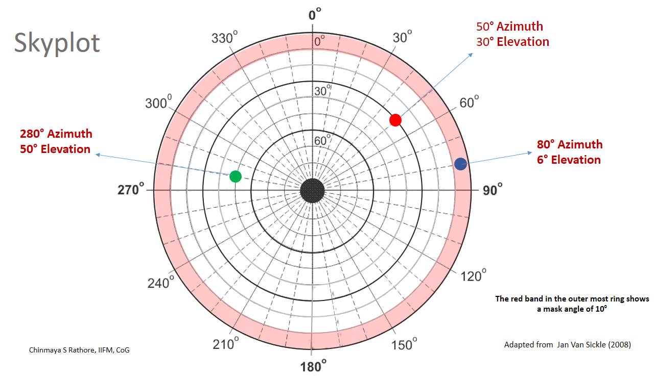
Now imagine that starting with the brown circle in figure 2 (which represents the horizon at the base of the dome), if we were to draw a circle around the blue dome upwards at every 10° elevation converging towards the zenith, we would have nine circles of elevation right up to 80° much like latitude lines on an earth globe. If we looked down from zenith, the arrangement would appears as shown in figure 3. The outermost dark ring in figure 3 represents the horizon (0° Elevation); the next lighter ring represents 10° elevation, the next 20° and so on until the innermost ring, which depicts 80° elevation. The dashed lines radiating out of the centre point represent the azimuth at 10° interval. The ensuing diagram as shown in figure 3 is a skyplot. The red dot is a satellite located at 50° azimuth and 30° elevation. The satellite indicated by the green dot is likewise at 280° azimuth and 50° elevation. The red band in figure 3 is the area between 0 - 10° elevation and it depicts a mask angle of 10°. The satellite shown by the blue dot located at 80° azimuth and 6° elevation falls inside the mask angle. When satellites on the skyplot shown as dots or some symbols (like in figure 1) are close together on the skyplot, you have poor geometry and higher DOPs. On the other hand, when the dots are far apart, there is good geometry and therefore lower DOPs.
Figure 3
Now that we are familiar with the Skyplot, let us look at a great software by GPS major Trimble called GNSS Planning Online (also available from this link ). Sometime back, this software was available as a standalone download to run on your computer. In that arrangement, the user had to get the latest almanac for this software to work. By making this software available online, Trimble automatically ensures that the latest almanacs are available to this software (figure 4) and the user can directly start working with the software. It needs to be mentioned that what this software is able to provide is possible only because of the availability of the almanac, which permits it to compute probable locations of GPS satellites at a particular time. Recall from part 1 of this article that almanacs store coarse orbital information of all satellites in the GPS constellation and the receiver (or a software for that matter) can use the almanac to locate satellites.
Figure 4
When you open the Trimble GNSS planning tool site, you might see a notification informing that you need to activate Silverlight, a plugin required to run this software. Click on the activate Silverlight link and you should see the landing page of the software shown in figure 5.
Figure 5
After you have filled in the requisite information in the settings page, you can choose from a number of displays by clicking other buttons in the left pane. The general idea is that on the settings screen, you first enter the latitude and longitude (type or pick using a map) of a point in the area where you are planning to conduct your GPS survey. You then choose an elevation mask (mentioned as cutoff on the screen), choose the time and date when you plan to conduct your GPS survey, choose your time zone and press apply. The Trimble GNSS planning tool will use the almanac to find out visibility of GPS satellites during the specified period, create a skyplot, and compute DOPs (figure 6).
Figure 6
Looking at the DOP graph, which shows GDOP, TDOP, HDOP, VDOP and PDOP, you can then choose a time window to conduct your survey where the PDOP or HDOP values are at their lowest and well within acceptable norms (PDOP of <= 4 and HDOP of <= 2 are excellent). The software also permits the user to look at disturbances in the form of Total Electron Content and Scintillation (see supplementary notes). Unfortunately, this software does not come with any help and assumes that user has understanding about the concept of DOPs, skyplots and almanacs. The primary purpose of providing the reader with conceptual background in this three-part article was to provide the requisite conceptual background necessary for using this software.As there are a some other important options available in the planning tool, I have created a full-length video tutorial on the use of this software for planning GPS surveys.
While there could be many other things that might be useful in planning GPS surveys (apart from what has been covered in this article series), the main objective of this series was to provide the reader with enough background in an easy to understand style to enable them to get started on the Trimble online GNSS planning tool. I hope you found this three part article series useful.